A Brief History of Neural Nets and Deep Learning
The story of how neural nets evolved from the earliest days of AI to now.
Prologue: The Deep Learning Tsunami
“Deep Learning waves have lapped at the shores of computational linguistics for several years now, but 2015 seems like the year when the full force of the tsunami hit the major Natural Language Processing (NLP) conferences.” -Dr. Christopher D. Manning, Dec 2015 1
This may sound hyperbolic - to say the established methods of an entire field of research are quickly being superseded by a new discovery, as if hit by a research ‘tsunami’. But, this catastrophic language is appropriate for describing the meteoric rise of Deep Learning over the last several years - a rise characterized by drastic improvements over reigning approaches towards the hardest problems in AI, massive investments from industry giants such as Google, and exponential growth in research publications (and Machine Learning graduate students). Having taken several classes on Machine Learning, and even used it in undergraduate research, I could not help but wonder if this new ‘Deep Learning’ was anything fancy or just a scaled up version of the ‘artificial neural nets’ that were already developed by the late 80s. And let me tell you, the answer is quite a story - the story of not just neural nets, not just of a sequence of research breakthroughs that make Deep Learning somewhat more interesting than ‘big neural nets’ (that I will attempt to explain in a way that just about anyone can understand), but most of all of how several unyielding researchers made it through dark decades of banishment to finally redeem neural nets and achieve the dream of Deep Learning.
I am certainly not a foremost expert on this topic. In depth technical overviews with long lists of references written by those who actually made the field what it is include Yoshua Bengio's "Learning Deep Architectures for AI", Jürgen Schmidhuber's "Deep Learning in Neural Networks: An Overview" and LeCun et al.s' "Deep learning". In particular, this is mostly a history of research in the US/Canada AI community, and even there will not mention many researchers; a particularly in depth history of the field that covers these omissions is Jürgen Schmidhuber's "Deep Learning in Neural Networks: An Overview". I am also most certainly not a professional writer, and will cop to there being shorter and much less technical overviews written by professional writers such as Paul Voosen's "The Believers", John Markoff's "Scientists See Promise in Deep-Learning Programs" and Gary Marcus's "Is “Deep Learning” a Revolution in Artificial Intelligence?". I also will stay away from getting too technical here, but there is a plethora of tutorials on the internet on all the major topics covered in brief by me.
Any corrections would be appreciated, though I will note some ommisions are intentional since I want to try and keep this 'brief' and a good mix of simple technical explanations and storytelling.
This piece is an updated and expanded version of blog posts originally released in 2015 on www.andreykurenkov.com.
- Prologue: The Deep Learning Tsunami
- Part 1: The Beginnings (1950s-1980s)
- Part 2: Neural Nets Blossom (1980s-2000s)
- Part 3: Deep Learning (2000s-2010s)
- Epilogue: The Decade of Deep Learning
Part 1: The Beginnings (1950s-1980s)
The beginning of a story spanning half a century, about how we learned to make computers learn. In this part, we shall cover the birth of neural nets with the Perceptron in 1958, the AI Winter of the 70s, and neural nets’ return to popularity with backpropagation in 1986.
The Centuries Old Machine Learning Algorithm

Let’s start with a brief primer on what Machine Learning is. Take some points on a 2D graph, and draw a line that fits them as well as possible. What you have just done is generalized from a few example of pairs of input values (x) and output values (y) to a general function that can map any input value to an output value. This is known as linear regression, and it is a wonderful little 200 year old technique for extrapolating a general function from some set of input-output pairs. And here’s why having such a technique is wonderful: there is an incalculable number of functions that are hard to develop equations for directly, but are easy to collect examples of input and output pairs for in the real world - for instance, the function mapping an input of recorded audio of a spoken word to an output of what that spoken word is.
Linear regression is a bit too wimpy a technique to solve the problem of speech recognition, but what it does is essentially what supervised Machine Learning is all about: ‘learning’ a function given a training set of examples, where each example is a pair of an input and output from the function (we shall touch on the unsupervised flavor in a little while). In particular, machine learning methods should derive a function that can generalize well to inputs not in the training set, since then we can actually apply it to inputs for which we do not have an output. For instance, Google’s current speech recognition technology is powered by Machine Learning with a massive training set, but not nearly as big a training set as all the possible speech inputs you might task your phone with understanding.
This generalization principle is so important that there is almost always a test set of data (more examples of inputs and outputs) that is not part of the training set. The separate set can be used to evaluate the effectiveness of the machine learning technique by seeing how many of the examples the method correctly computes outputs for given the inputs. The nemesis of generalization is overfitting - learning a function that works really well for the training set but badly on the test set. Since machine learning researchers needed means to compare the effectiveness of their methods, over time there appeared standard datasets of training and testing sets that could be used to evaluate machine learning algorithms.
Okay okay, enough definitions. Point is - our line drawing exercise is a very simple example of supervised machine learning: the points are the training set (X is input and Y is output), the line is the approximated function, and we can use the line to find Y values for X values that don’t match any of the points we started with. Don’t worry, the rest of this history will not be nearly so dry as all this. Here we go.
The Folly of False Promises
Why have all this prologue with linear regression, since the topic here is ostensibly neural nets? Well, in fact linear regression bears some resemblance to the first idea conceived specifically as a method to make machines learn: Frank Rosenblatt’s Perceptron2.

A psychologist, Rosenblatt conceived of the Percetron as a simplified mathematical model of how the neurons in our brains operate: it takes a set of binary inputs (nearby neurons), multiplies each input by a continuous valued weight (the synapse strength to each nearby neuron), and thresholds the sum of these weighted inputs to output a 1 if the sum is big enough and otherwise a 0 (in the same way neurons either fire or do not). Most of the inputs to a Perceptron are either some data or the output of another Perceptron, but an extra detail is that Perceptrons also have one special ‘bias’ input, which just has a value of 1 and basically ensures that more functions are computable with the same input by being able to offset the summed value. This model of the neuron built on the work of Warren McCulloch and Walter Pitts Mcculoch-Pitts3, who showed that a neuron model that sums binary inputs and outputs a 1 if the sum exceeds a certain threshold value, and otherwise outputs a 0, can model the basic OR/AND/NOT functions. This, in the early days of AI, was a big deal - the predominant thought at the time was that making computers able to perform formal logical reasoning would essentially solve AI.
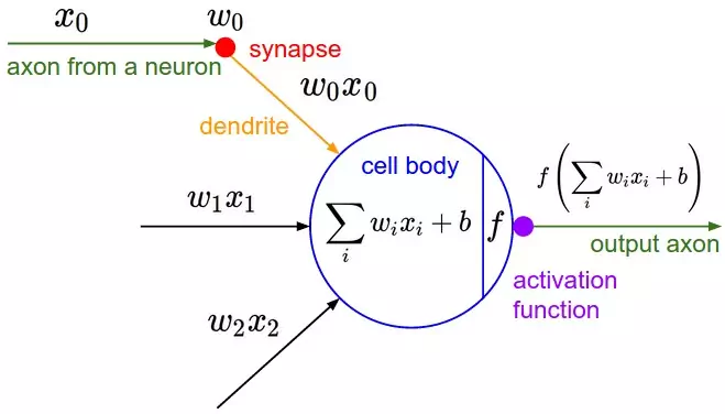
However, the Mcculoch-Pitts model lacked a mechanism for learning, which was crucial for it to be usable for AI. This is where the Perceptron excelled - Rosenblatt came up with a way to make such artificial neurons learn, inspired by the foundational work4 of Donald Hebb. Hebb put forth the unexpected and hugely influential idea that knowledge and learning occurs in the brain primarily through the formation and change of synapses between neurons - concisely stated as Hebb’s Rule:
“When an axon of cell A is near enough to excite a cell B and repeatedly or persistently takes part in firing it, some growth process or metabolic change takes place in one or both cells such that A’s efficiency, as one of the cells firing B, is increased.”
The Perceptron did not follow this idea exactly, but having weights on the inputs allowed for a very simple and intuitive learning scheme: given a training set of input-output examples the Perceptron should ‘learn’ a function from, for each example increase the weights if the Perceptron output for that example’s input is too low compared to the example, and otherwise decrease the weights if the output is too high. Stated ever so slightly more formally, the algorithm is as follows:
- Start off with a Perceptron having random weights and a training set
- For the inputs of an example in the training set, compute the Perceptron’s output
- If the output of the Perceptron does not match the output that is known to be correct for the example:
- If the output should have been 0 but was 1, decrease the weights that had an input of 1.
- If the output should have been 1 but was 0, increase the weights that had an input of 1.
- Go to the next example in the training set and repeat steps 2-4 until the Perceptron makes no more mistakes
This procedure is simple, and produces a simple result: an input linear function (the weighted sum), just as with linear regression, ‘squashed’ by a non-linear activation function (the thresholding of the sum). It’s fine to threshold the sum when the function can only have a finite set of output values (as with logical functions, in which case there are only two - True/1 and False/0), and so the problem is not so much to generate a continuous-numbered output for any set of inputs - regression - as to categorize the inputs with a correct label - classification.
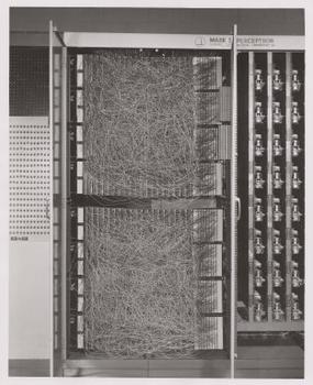
Rosenblatt implemented the idea of the Perceptron in custom hardware (this being before fancy programming languages were in common use), and showed it could be used to learn to classify simple shapes correctly with 20x20 pixel-like inputs. And so, machine learning was born - a computer was built that could approximate a function given known input and output pairs from it. In this case it learned a little toy function, but it was not difficult to envision useful applications such as converting the mess that is human handwriting into machine-readable text.
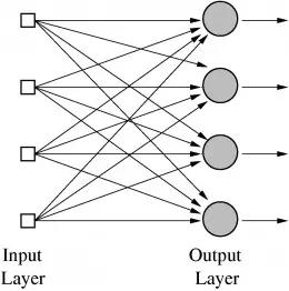
But wait, so far we’ve only seen how one Perceptron is able to learn to output a one or a zero - how can this be extended to work for classification tasks with many categories, such as human handwriting (in which there are many letters and digits as the categories)? This is impossible for one Perceptron, since it has only one output, but functions with multiple outputs can be learned by having multiple Perceptrons in a layer, such that all these Perceptrons receive the same input and each one is responsible for one output of the function. Indeed, neural nets (or, formally, ‘Artificial Neural Networks’ - ANNs) are nothing more than layers of Perceptrons - or neurons, or units, as they are usually called today - and at this stage there was just one layer - the output layer. So, a prototypical example of neural net use is to classify an image of a handwritten digit. The inputs are the pixels of the image , and there are 10 output neurons with each one corresponding to one of the 10 possible digit values. In this case only one of the 10 neurons output 1, the highest weighted sum is taken to be the correct output, and the rest output 0.
It is also possible to conceive of neural nets with artificial neurons different from the Perceptron. For instance, the thresholding activation function is not strictly necessary; Bernard Widrow and Tedd Hoff soon explored the option of just outputting the weight input in 1960 with “An adaptive “ADALINE” neuron using chemical “memistors”5, and showed how these ‘Adaptive Linear Neurons’ could be incorporated into electrical circuits with ‘memistors’ - resistors with memory. They also showed that not having the threshold activation function is mathematically nice, because the neuron’s learning mechanism can be formally based on minimizing the error through good ol’ calculus. See, with the neuron’s function not being made weird by this sharp thresholding jump from 0 to 1, a measure of how much the error changes when each weight is changed (the derivative) can be used to drive the error down and find the optimal weight values. As we shall see, finding the right weights using the derivatives of the training error with respect to each weight is exactly how neural nets are typically trained to this day.
In short a function is differentiable if it is a nice smooth line - Rosenblatt's Perceptron computed the output in such a way that the output abruptly jumped from 0 to 1 if the input exceeded some number, whereas Adaline simply output the input which was a nice non-jumpy line. For a much more in depth explanation of all this math you can read this tutorial, or any resource from Google - let us focus on the fun high-level concepts and story here.
If we think about ADALINE a bit more we will come up with a further insight: finding a set of weights for a number of inputs is really just a form of linear regression. And again, as with linear regression, this would not be enough to solve the complex AI problems of Speech Recognition or Computer Vision. What McCullough and Pitts and Rosenblatt were really excited about is the broad idea of Connectionism: that networks of such simple computational units can be vastly more powerful and solve the hard problems of AI. And, Rosenblatt said as much, as in this frankly ridiculous New York Times quote from the time6:
“The Navy revealed the embryo of an electronic computer today that it expects will be able to walk, talk, see, write, reproduce itself an be conscious of its existence … Dr. Frank Rosenblatt, a research psychologist at the Cornell Aeronautical Laboratory, Buffalo, said Perceptrons might be fired to the planets as mechanical space explorers”
Or, have a look at this TV segment from the time:
This sort of talk no doubt irked other researchers in AI, many of whom were focusing on approaches based on manipulation of symbols with concrete rules that followed from the mathematical laws of logic. Marvin Minsky, founder of the MIT AI Lab, and Seymour Papert, director of the lab at the time, were some of the researchers who were skeptical of the hype and in 1969 published their skepticism in the form of rigorous analysis on of the limitations of Perceptrons in a seminal book aptly named Perceptrons7. Interestingly, Minksy may have actually been the first researcher to implement a hardware neural net with 1951’s SNARC (Stochastic Neural Analog Reinforcement Calculator) 8, which preceded Rosenblatt’s work by many years. But the lack of any trace of his work on this system and the critical nature of the analysis in Perceptrons suggests that he concluded this approach to AI was a dead end. The most widely discussed element of this analysis is the elucidation of the limits of a Perceptron - they could not, for instance, learn the simple boolean function XOR because it is not linearly separable. Though the history here is vague, this publication is widely believed to have helped usher in the first of the AI Winters - a period following a massive wave of hype for AI characterized by disillusionment that causes a freeze to funding and publications.

The Thaw of the AI Winter
So, things were not good for neural nets. But why? The idea, after all, was to combine a bunch of simple mathematical neurons to do complicated things, not to use a single one. In other terms, instead of just having one output layer, to send an input to arbitrarily many neurons which are called a hidden layer because their output acts as input to another hidden layer or the output layer of neurons. Only the output layer’s output is ‘seen’ - it is the answer of the neural net - but all the intermediate computations done by the hidden layer(s) can tackle vastly more complicated problems than just a single layer.
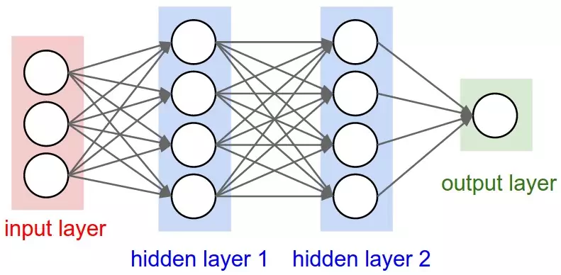
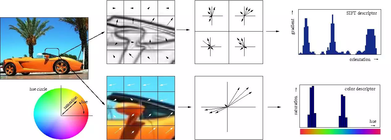
The reason hidden layers are good, in basic terms, is that the hidden layers can find features within the data and allow following layers to operate on those features rather than the noisy and large raw data. For example, in the very common neural net task of finding human faces in an image, the first hidden layer could take in the raw pixel values and find lines, circles, ovals, and so on within the image. The next layer would receive the position of these lines, circles, ovals, and so on within the image and use those to find the location of human faces - much easier! And people, basically, understood this. In fact, until recently machine learning techniques were commonly not applied directly to raw data inputs such as images or audio. Instead, machine learning was done on data after it had passed through feature extraction - that is, to make learning easier machine learning was done on preprocessed data from which more useful features such as angles or shapes had been already extracted.
Earlier, we saw that the weighted sum computed by the Perceptron is usually put through a non-linear activation function. Now we can get around to fully answering an implicit question: why bother? Two reasons: 1. Without the activation function, the learned functions could only be linear, and most 'interesting' functions are not linear (for instance, logic functions that only output 1 or 0 or classification functions that output the category). 2. Several layers of linear Perceptrons can always be collapsed into only one layer due to the linearity of all the computations - the same cannot be done with non-linear activation functions.
So, in intuitive speak a network can massage the data better with activation functions than without.
So, it is important to note Minsky and Papert’s analysis of Perceptrons did not merely show the impossibility of computing XOR with a single Perceptron, but specifically argued that it had to be done with multiple layers of Perceptrons - what we now call multilayer neural nets - and that Rosenblatt’s learning algorithm did not work for multiple layers. And that was the real problem: the simple learning rule previously outlined for the Perceptron does not work for multiple layers. To see why, let’s reiterate how a single layer of Perceptrons would learn to compute some function:
- A number of Perceptrons equal to the number of the function’s outputs would be started off with small initial weights
- For the inputs of an example in the training set, compute the Perceptrons’ output
- For each Perceptron, if the output does not match the example’s output, adjust the weights accordingly
- Go to the next example in the training set and repeat steps 2-4 until the Perceptrons no longer make mistakes
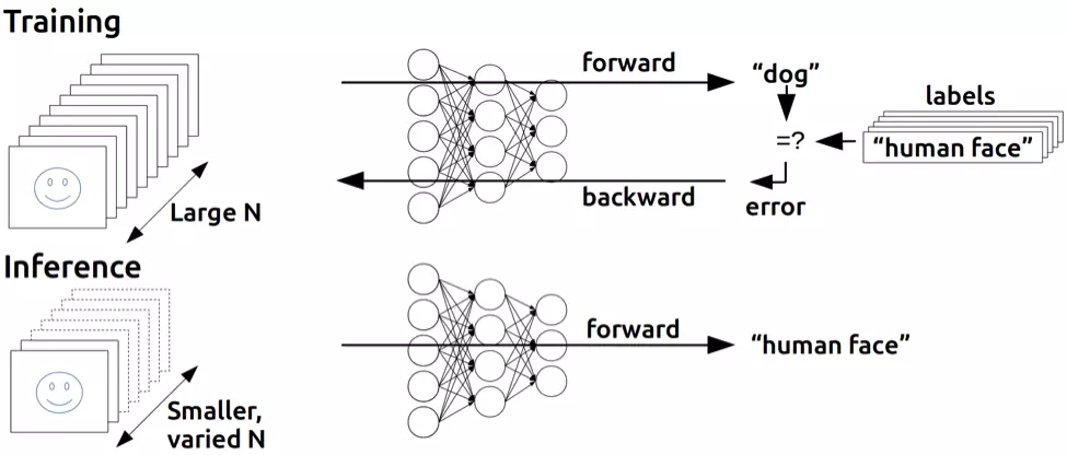
The reason why this does not work for multiple layers should be intuitively clear: the example only specifies the correct output for the final output layer, so how in the world should we know how to adjust the weights of Perceptrons in layers before that? The answer, despite taking some time to derive, proved to be once again based on age-old calculus: the chain rule. The key realization was that if the neural net neurons were not quite Perceptrons, but were made to compute the output with an activation function that was still non-linear but also differentiable, as with Adaline, not only could the derivative be used to adjust the weight to minimize error, but the chain rule could also be used to compute the derivative for all the neurons in a prior layer and thus the way to adjust their weights would also be known. Or, more simply: we can use calculus to assign some of the blame for any training set mistakes in the output layer to each neuron in the previous hidden layer, and then we can further split up blame if there is another hidden layer, and so on - we backpropagate the error. And so, we can find how much the error changes if we change any weight in the neural net, including those in the hidden layers, and use an optimization technique (for a long time, typically stochastic gradient descent) to find the optimal weights to minimize the error.
Backpropagation was derived by multiple researchers in the early 60’s and implemented to run on computers much as it is today as early as 1970 by Seppo Linnainmaa9, but Paul Werbos was first in the US to propose that it could be used for neural nets after analyzing it in depth in his 1974 PhD Thesis10. Interestingly, as with Perceptrons he was loosely inspired by work modeling the human mind, in this case the psychological theories of Freud as he himself recounts11:
“In 1968, I proposed that we somehow imitate Freud’s concept of a backwards flow of credit assignment, flowing back from neuron to neuron … I explained the reverse calculations using a combination of intuition and examples and the ordinary chainrule, though it was also exactly a translation into mathematics of things that Freud had previously proposed in his theory of psychodynamics!”
Despite solving the question of how multilayer neural nets could be trained, and seeing it as such while working on his PhD thesis, Werbos did not publish on the application of backprop to neural nets until 1982 due to the chilling effects of the AI Winter. In fact, Werbos thought the approach would make sense for solving the problems pointed out in Perceptrons, but the community at large lost any faith in tackling those problems:
“Minsky’s book was best known for arguing that (1) we need to use MLPs [multilayer perceptrions, another term for multilayer neural nets] even to represent simple nonlinear functions such as the XOR mapping; and (2) no one on earth had found a viable way to train MLPs good enough to learn such simple functions. Minsky’s book convinced most of the world that neural networks were a discredited dead-end – the worst kind of heresy. Widrow has stressed that this pessimism, which squashed the early “perceptron” school of AI, should not really be blamed on Minsky. Minsky was merely summarizing the experience of hundreds of sincere researchers who had tried to find good ways to train MLPs, to no avail. There had been islands of hope, such as the algorithm which Rosenblatt called “backpropagation” (not at all the same as what we now call backpropagation!), and Amari’s brief suggestion that we might consider least squares [what is the basis of simple linear regression] as a way to train neural networks (without discussion of how to get the derivatives, and with a warning that he did not expect much from the approach). But the pessimism at that time became terminal. In the early 1970s, I did in fact visit Minsky at MIT. I proposed that we do a joint paper showing that MLPs can in fact overcome the earlier problems … But Minsky was not interested(14). In fact, no one at MIT or Harvard or any place I could find was interested at the time.”
It seems that it was because of this lack of academic interest that it was not until more than a decade later, in 1986, that this approach was popularized in “Learning representations by back-propagating errors” by David Rumelhart, Geoffrey Hinton, and Ronald Williams 12. Despite the numerous discoveries of the method (the paper even explicitly mentions David Parker and Yann LeCun as two people who discovered it beforehand) the 1986 publication stands out for how concisely and clearly the idea is stated. In fact, as a student of Machine Learning it is easy to see that the description in their paper is essentially identical to the way the concept is still explained in textbooks and AI classes. A retrospective in IEEE13 echoes this notion:
“Unfortunately, Werbos’s work remained almost unknown in the scientific community. In 1982, Parker rediscovered the technique [39] and in 1985, published a report on it at M.I.T. [40]. Not long after Parker published his findings, Rumelhart, Hinton, and Williams [41], [42] also rediscovered the techniques and, largely as a result of the clear framework within which they presented their ideas, they finally succeeded in making it widely known.”
But the three authors went much further than just present this new learning algorithm. In the same year they published the much more in-depth “Learning internal representations by error propagation”14, which specifically addressed the problems discussed by Minsky in Perceptrons. Though the idea was conceived by people in the past, it was precisely this formulation in 1986 that made it widely understood how multilayer neural nets could be trained to tackle complex learning problems. And so, neural nets were back! Next, we shall see how just a few years later backpropagation and some other tricks discussed in “Learning internal representations by error propagation” were applied to a very significant problem: enabling computers to read human handwriting.
Part 2: Neural Nets Blossom (1980s-2000s)
Neural Nets Gain Vision
With the secret to training multilayer neural nets uncovered, the topic was once again ember-hot and the lofty ambitions of Rosenblatt seemed to perhaps be in reach. It took only until 1989 for another key finding now universally cited in textbooks and lectures to be published15: “Multilayer feedforward networks are universal approximators”. Essentially, it mathematically proved that multiple layers allow neural nets to theoretically implement any function, and certainly XOR.
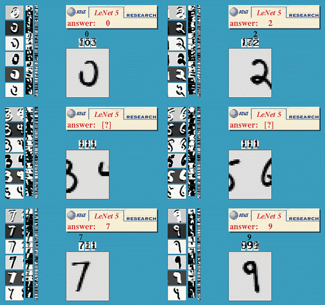
But, this is mathematics, where you could imagine having endless memory and computation power should it be needed - did backpropagation allow neural nets to be used for anything in the real world? Oh yes. Also in 1989, Yann LeCun et al. at the AT&T Bell Labs demonstrated a very significant real-world application of backpropagation in "”Backpropagation Applied to Handwritten Zip Code Recognition” 16. You may think it fairly unimpressive for a computer to be able to correctly understand handwritten digits, and these days it is indeed quite quaint, but prior to the publication the messy and inconsistent scrawls of us humans proved a major challenge to the much more tidy minds of computers. The publication, working with a large dataset from the US Postal Service, showed neural nets were entirely capable of this task. And much more importantly, it was first to highlight the practical need for a key modifications of neural nets beyond plain backpropagation toward modern deep learning:
“Classical work in visual pattern recognition has demonstrated the advantage of extracting local features and combining them to form higher order features. Such knowledge can be easily built into the network by forcing the hidden units to combine only local sources of information. Distinctive features of an object can appear at various location on the input image. Therefore it seems judicious to have a set of feature detectors that can detect a particular instance of a feature anywhere on the input place. Since the precise location of a feature is not relevant to the classification, we can afford to lose some position information in the process. Nevertheless, approximate position information must be preserved, to allow the next levels to detect higher order, more complex features (Fukushima 1980; Mozer 1987).”
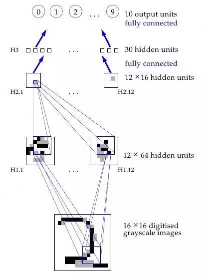
Or, more concretely: the first hidden layer of the neural net was convolutional - instead of each neuron having a different weight for each pixel of the input image (40x60=2400 weights), the neurons only have a small set of weights (5x5=25) that were applied a whole bunch of small subsets of the image of the same size. So, for instance instead of having 4 different neurons learn to detect 45 degree lines in each of the 4 corners of the input image, a single neuron could learn to detect 45 degree lines on subsets of the image and do that everywhere within it. Layers past the first work in a similar way, but take in the ‘local’ features found in the previous hidden layer rather than pixel images, and so ‘see’ successively larger portions of the image since they are combining information about increasingly larger subsets of the image. Finally, the last two layers are just plain normal neural net layers that use the higher-order larger features generated by the convolutional layers to determine which digit the input image corresponds to. The method proposed in this 1989 paper went on to be the basis of nationally deployed check-reading systems, as demonstrated by LeCun in this gem of a video:
The reason for why this is helpful is intuitively if not mathematically clear: without such constraints the network would have to learn the same simple things (such as detecting 45 degree lines, small circles, etc) a whole bunch of times for each portion of the image. But with the constraint there, only one neuron would need to learn each simple feature - and with far fewer weights overall, it could do so much faster! Moreover, since the pixel-exact locations of such features do not matter the neuron could basically skip neighboring subsets of the image - subsampling, now known as a type of pooling - when applying the weights, further reducing the training time. The addition of these two types of layers - convolutional and pooling layers - are the primary distinctions of Convolutional Neural Nets (CNNs/ConvNets) from plain old neural nets.
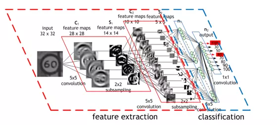
At that time, the convolution idea was called ‘weight sharing’, and it was actually discussed in the 1986 extended analysis of backpropagation by Rumelhart, Hinton, and Williams17. Actually, the credit goes even further back - Minsky and Papert’s 1969 analysis of Perceptrons was thorough enough to pose a problem that motivated this idea. But, as before, others have also independently explored the concept - namely, Kunihiko Fukushima in 1980 with his notion of the Neurocognitron18. And, as before, the ideas behind it drew inspiration from studies of the brain:
“According to the hierarchy model by Hubel and Wiesel, the neural network in the visual cortex has a hierarchy structure: LGB (lateral geniculate body)->simple cells->complex cells->lower order hypercomplex cells->higher order hypercomplex cells. It is also suggested that the neural network between lower order hypercomplex cells and higher order hypercomplex cells has a structure similar to the network between simple cells and complex cells. In this hierarchy, a cell in a higher stage generally has a tendency to respond selectively to a more complicated feature of the stimulus pattern, and, at the same time, has a larger receptive field, and is more insensitive to the shift in position of the stimulus pattern. … Hence, a structure similar to the hierarchy model is introduced in our model.”
LeCun continued to be a major proponent of CNNs at Bell Labs, and his work on them resulted in major commercial use for check-reading in the mid 90s - his talks and interviews often include the fact that “At some point in the late 1990s, one of these systems was reading 10 to 20% of all the checks in the US.”19.
Neural Nets Go Unsupervised
Automating the rote and utterly uninteresting task of reading checks is a great instance of what Machine Learning can be used for. Perhaps a less predictable application? Compression. Meaning, of course, finding a smaller representation of some data from which the original data can be reconstructed. Learned compression may very well outperform stock compression schemes, when the learning algorithm can find features within the data stock methods would miss. And it is very easy to do - just train a neural net with a small hidden layer to just output the input:
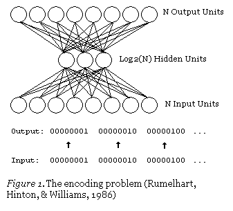
This is an autoencoder neural net, and is a method for learning compression - efficiently translating (encoding) data to a compact format and back to itself (auto). See, the output layer computes its outputs, which ideally are the same as the input to the neural net, using only the hidden layer’s outputs. Since the hidden layer has fewer outputs than does the input layer, the output of the hidden layer is the compressed representation of the input data, which can be reconstructed with the output layer.
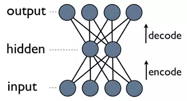
Notice a neat thing here: the only thing we need for training is some input data. This is in contrast to the requirement of supervised machine learning, which needs a training set of input-output pairs (labeled data) in order to approximate a function that can compute such outputs from such inputs. And indeed, autoencoders are not a form of supervised learning; they are a form of unsupervised learning, which only needs a set of input data (unlabeled data) in order to find some hidden structure within that data. In other words, unsupervised learning does not approximate a function so much as it derives one from the input data to another useful representation of that data. In this case, this representation is just a smaller one from which the original data can still be reconstructed, but it can also be used for finding groups of similar data (clustering) or other inference of latent variables (some aspect that is known to exist for the data but the value of which is not known).
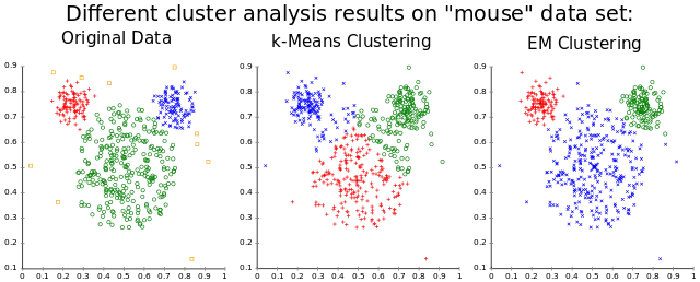
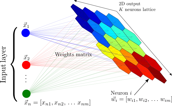
There were other unsupervised applications of neural networks explored prior to and after the discovery of backpropagation, most notably Self Organizing Maps 20, which produce a low-dimensional representation of data good for visualization, and Adapative Resonance Theory21, which can learn to classify arbitrary input data without being told correct classifications. If you think about it, it is intuitive that quite a lot can be learned from unlabeled data. Say you have a dataset of a bunch of images of handwritten digits, without labels of which digit each image corresponds to. Well, an image with some digit in that dataset most likely looks most like all the other images with that same digit, and so though a computer may not know which digit all those images correspond to, it should still be able to find that they all correspond to the same one. This, pattern recognition, is really what most of machine learning is all about, and arguably also is the basis for the great powers of the human brain. But, let us not digress from our exciting deep learning journey, and get back to autoencoders.
As with weight-sharing, the idea of autoencoders was first discussed in the aforementioned extensive 1986 analysis of backpropagation 17, and as with weight-sharing it resurfaced in more research in the following years2223, including by Hinton himself 24. This paper, with the fun title “Autoencoders, Minimum Description Length, and Helmholts Free Energy”, posits that “A natural approach to unsupervised learning is to use a model that defines probability distribution over observable vectors” and uses a neural net to learn such a model. So here’s another neat thing you can do with neural nets: approximate probability distributions.
Neural Nets Gain Beliefs
In fact, before being co-author of the seminal 1986 paper on backpropagation learning algorithm, Hinton worked on a neural net approach for learning probability distributions in the 1985 “A Learning Algorithm for Boltzmann Machines” 25. Boltzmann Machines are networks just like neural nets and have units that are very similar to Perceptrons, but instead of computing an output based on inputs and weights, each unit in the network can compute a probability of it having a value of 1 or 0 given the values of connected units and weights. The units are therefore stochastic - they behave according to a probability distribution, rather than in a known deterministic way. The Boltzmann part refers to a probability distribution that has to do with the states of particles in a system based the particles’ energy and on the thermodynamic temperature of that system. This distribution defines not only the mathematics of the Boltzmann machines, but also the interpretation - the units in the network themselves have energies and states, and learning is done by minimizing the energy of the system - a direct inspiration from thermodynamics. Though a bit unintuitive, this energy-based interpretation is actually just one example of an energy-based model, and fits in the energy-based learning theoretical framework with which many learning algorithms can be expressed26.
That there is a common theoretical framework for a bunch of learning methods is not too surprising, since at the end of the day all of learning boils down to optimization. Quoting from the above cited tutorial:
"Training an EBM consists in finding an energy function that produces the best Y for any X ... The architecture of the EBM is the internal structure of the parameterized energy function E(W, Y, X) ... This quality measure is called the loss functional (i.e. a function of function) and denoted L(E,S). ... In order to find the best energy function [] we need a way to assess the quality of any particular energy function, based solely on two elements: the training set, and our prior knowledge about the task. For simplicity, we often denote it L(W,S) and simply call it the loss function. The learning problem is simply to find the W that minimizes the loss."
So, the key to energy based models is recognizing all these algorithms are essentially different ways to optimize a pair of functions, that can be called the energy function E and loss function L, by finding a set of good values to a bunch of variables that can be denoted W using data denoted X for input and Y for the output. It's really a very broad definition for a framework, but still nicely encapsulates what a lot of algorithms fundamentally do.

Back to Boltzmann Machines. When such units are put together into a network, they form a graph, and so are a graphical model of data. Essentially, they can do something very similar to normal neural nets: some hidden units compute the probability of some hidden variables (the outputs - classifications or features for data) given known values of visible units that represent visible variables (the inputs - pixels of images, characters in text, etc.). In our classic example of classifying images of digits, the hidden variables are the actual digit values, and the visible variables are the pixels of the image; given an image of the digit ‘1’ as input, the value of visible units is known and the hidden unit modeling the probability of the image representing a ‘1’ should have a high output probability.
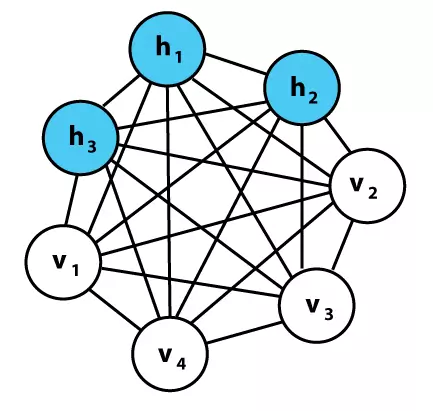
So, for the classification task, there is now a nice way of computing the probability of each category. This is very analogous to actually computing the output values of a normal classification neural net, but these nets have another neat trick: they can generate plausible looking input data. This follows from the probability equations involved - not only does the net learn the probabilities of values for the hidden variables given known values for the visible variables, but also the inverse of that - visible probabilities given known hidden values. So, if we want to generate a ‘1’ digit image, the units corresponding to the pixel variables have known probabilities of outputting a 1 and an image can be probabilistically generated; these networks are generative graphical models. Though it is possible to do supervised learning with very similar goals as normal neural nets, the unsupervised learning task of learning a good generative model - probabilistically learning the hidden structure of some data - is commonly what these nets are used for. Most of this was not really that novel, but the learning algorithm presented and the particular formulation that enabled it were, as stated in the paper itself:
“Perhaps the most interesting aspect of the Boltzmann Machine formulation is that it leads to a domain-independent learning algorithm that modifies the connection strengths between units in such a way that the whole network develops an internal model which captures the underlying structure of its environment. There has been a long history of failure in the search for such algorithms (Newell, 1982), and many people (particularly in Artificial Intelligence) now believe that no such algorithms exist.”
Having learned the classical neural net models first, it took me a while to understand the notion behind these probabilistic nets. To elaborate, let me present a quote from the paper itself that restates all that I have said above quite well:
"The network modifies the strengths of its connections so as to construct an internal generative model that produces examples with the same probability distribution as the examples it is shown. Then, when shown any particular example, the network can “interpret” it by finding values of the variables in the internal model that would generate the example.
...
The machine is composed of primitive computing elements called units that are connected to each other by bidirectional links. A unit is always in one of two states, on or off, and it adopts these states as a probabilistic function of the states of its neighboring units and the weights on its links to them. The weights can take on real values of either sign. A unit being on or off is taken to mean that the system currently accepts or rejects some elemental hypothesis about the domain. The weight on a link represents a weak pairwise constraint between two hypotheses. A positive weight indicates that the two hypotheses tend to support one another; if one is currently accepted, accepting the other should be more likely. Conversely, a negative weight suggests, other things being equal, that the two hypotheses should not both be accepted. Link weights are symmetric, having the same strength in both directions (Hinton & Sejnowski, 1983)."
Without delving into the full details of the algorithm, here are some highlights: it is a variant on maximum-likelihood algorithms, which simply means that it seeks to maximize the probability of the net’s visible unit values matching with their known correct values. Computing the actual most likely value for each unit all at the same time turns out to be much too computationally expensive, so in training Gibbs Sampling - starting the net with random unit values and iteratively reassigning values to units given their connections’ values - is used to give some actual known values. When learning using a training set, the visible units are just set to have the value of the current training example, so sampling is done to get values for the hidden units. Once some ‘real’ values are sampled, we can do something similar to backpropagation - take a derivative for each weight to see how we can change so as to increase the probability of the net doing the right thing.
As with neural net, the algorithm can be done both in a supervised fashion (with known values for the hidden units) or in an unsupervised fashion. Though the algorithm was demonstrated to work (notably, with the same ‘encoding’ problem that autoencoder neural nets solve), it was soon apparent that it just did not work very well - Redford M. Neal’s 1992 “Connectionist learning of belief networks”27 justified a need for a faster approach by stating that: “These capabilities would make the Boltzmann machine attractive in many applications, were it not that its learning procedure is generally seen as being painfully slow”. And so Neal introduced a similar idea in the belief net, which is essentially like a Boltzmann machine with directed, forward connections (so that there are again layers, as with the the neural nets we have seen before, and unlike the Boltzmann machine image above). Without getting into mucky probability math, this change allowed the nets to be trained with a faster learning algorithm. We actually saw a ‘belief net’ just above with the sprinkler and rain variables, and the term was chosen precisely because this sort of probability-based modeling has a close relationship to ideas from the mathematical field of probability, in addition to its link to the field of Machine Learning.
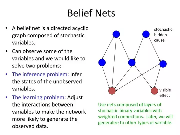
Though this approach was an advance upon Boltzmann machines, it was still just too slow - the math for correctly deriving probabilistic relations between variables is such that a ton of computation is typically required without some simplifying tricks. And so Hinton, along with Neal and two other co-authors, soon came up with extra tricks in the 1995 “The wake-sleep algorithm for unsupervised neural networks”28. These tricks called for a slightly different belief net setup, which was now deemed “The Helmholtz Machine”29. Skirting the details once again, the key idea was to have separate sets of weights for inferring hidden variables from visible variables (recognition weights) and vice versa (generative weights), and to keep the directed aspect of Neal’s belief nets. This allows the training to be done much faster, while being applicable to the unsupervised and supervised learning problems of Boltzmann Machines.
In videos of Hinton talking about the Wake Sleep algorithm, he often notes how gross the simplifying assumption being made is, and that it turns out the algorithm just works regardless. Again I will quote as the paper itself explains the assumption well:
"The key simplifying assumption is that the recognition distribution for a particular example d, Q is factorial (separable) in each layer. If there are h stochastic binary units in a layer B, the portion of the distribution P(B,d) due to that layer is determined by 2^(h - 1) probabilities. However, Q makes the assumption that the actual activity of any one unit in layer P is independent of the activities of all the other units in that layer, given the activities of all the units in the lower layer, l - 1, so the recognition model needs only specify h probabilities rather than 2" - 1. The independence assumption allows F(d; 8.4) to be evaluated efficiently, but this computational tractability is bought at a price, since the true posterior is unlikely to be factorial
...
The generative model is taken to be factorial in the same way, although one should note that factorial generative models rarely have recognition distributions that are themselves exactly factorial."
Note the Neal's belief nets also implicitly made the probabilities factorize by having layers of units with only forward-facing directed connections.
Finally, belief nets could be trained somewhat fast! Though not quite as influential, this algorithmic advance was a significant enough forward step for unsupervised training of belief nets that it could be seen as a companion to the now almost decade-old publication on backpropagation. But, by this point new machine learning methods had begun to also emerge, and people were again beginning to be skeptical of neural nets since they seemed so intuition-based and since computers were still barely able to meet their computational needs. As we’ll soon see, a new AI Winter for neural nets began just a few years later…
Neural Nets Make Decisions
Having discovered the application of neural nets to unsupervised learning, let us also quickly see how they were used in the third branch of machine learning: reinforcement learning. This one requires the most mathy notation to explain formally, but also has a goal that is very easy to describe informally: learn to make good decisions. Given some theoretical agent (a little software program, for instance), the idea is to make that agent able to decide on an action based on its current state, with the reception of some reward for each action and the intent of getting the maximum utility in the long term. So, whereas supervised learning tells the learning algorithm exactly what it should learn to output, reinforcement learning provides ‘rewards’ as a by-product of making good decisions over time, and does not directly tell the algorithm the correct decisions to choose. From the outset it was a very abstracted decision making model - there were a finite number of states, and a known set of actions with known rewards for each state. This made it easy to write very elegant equations for finding the optimal set of actions, but hard to apply to real problems - problems with continuous states or hard-to-define rewards.
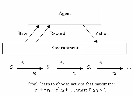
This is where neural nets come in. Machine learning in general, and neural nets in particular, are good at dealing with messy continuous data or dealing with hard to define functions by learning them from examples. Although classification is the bread and butter of neural nets, they are general enough to be useful for many types of problems - the descendants of Bernard Widrow’s and Ted Hoff’s Adaline were used for adaptive filters in the context of electrical circuits, for instance. And so, following the resurgence of research caused by backpropagation, people soon devised ways of leveraging the power of neural nets to perform reinforcement learning. One of the early examples of this was solving a simple yet classic problem: the balancing of a stick on a moving platform, known to students in control classes everywhere as the inverted pendulum problem 30.
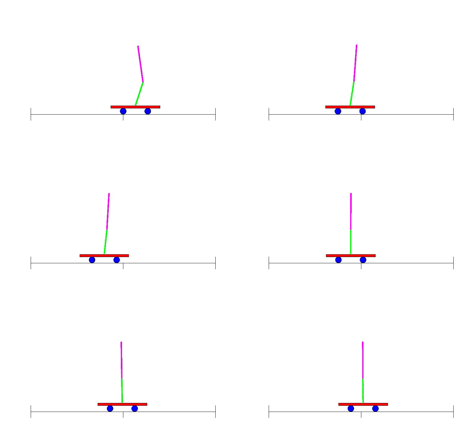
As with adaptive filtering, this research was strongly relevant to the field of Electrical Engineering, where control theory had been a major subfield for many decades prior to neural nets’ arrival. Though the field had devised ways to deal with many problems through direct analysis, having a means to deal with more complex situations through learning proved useful as evidenced by the hefty 7000 (!) citations of the 1990 “Identification and control of dynamical systems using neural networks”31. Perhaps predictably, there was another field separate from Machine Learning where neural nets were useful - robotics. A major example of early neural net use for robotics came from CMU’s NavLab with 1989’s “Alvinn: An autonomous land vehicle in a neural network”32:
As discussed in the paper, the neural net in this system learned to control the vehicle through plain supervised learning using sensor and steering data recorded while a human drove. There was also research into teaching robots using reinforcement learning specifically, as exemplified by the 1993 PhD thesis “Reinforcement learning for robots using neural networks”33. The thesis showed that robots could be taught behaviors such as wall following and door passing in reasonable amounts of time, which was a good thing considering the prior inverted pendulum work requires impractical lengths of training.
These disparate applications in other fields are certainly cool, but of course the most research on reinforcement learning and neural nets was happening within AI and Machine Learning. And here, one of the most significant results in the history of reinforcement learning was achieved: a neural net that learned to be a world class backgammon player. Dubbed TD-Gammon, the neural net was trained using a standard reinforcement learning algorithm and was one of the first demonstrations of reinforcement learning being able to outperform humans on relatively complicated tasks 34. And it was specifically a reinforcement learning approach that worked here, as the same research showed just using a neural net without reinforcement learning did not work nearly as well.
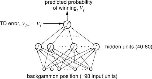
But, as we have seen happen before and will see happen again in AI, research hit a dead end. The predictable next problem to tackle using the TD-Gammon approach was investigated by Sebastian Thrun in the 1995 “Learning To Play the Game of Chess”, and the results were not good 35. Though the neural net learned decent play, certainly better than a complete novice at the game, it was still far worse than a standard computer program (GNU-Chess) implemented long before. The same was true for the other perennial challenge of AI, Go 36. See, TD-Gammon sort of cheated - it learned to evaluate positions quite well, and so could get away with not doing any ‘search’ over multiple future moves and instead just picking the one that led to the best next position. But the same is simply not possible in chess or Go, games which are a challenge to AI precisely because of needing to look many moves ahead and having so many possible move combinations. Besides, even if the algorithm were smarter, the hardware of the time just was not up to the task - Thrun reported that “NeuroChess does a poor job, because it spends most of its time computing board evaluations. Computing a large neural network function takes two orders of magnitude longer than evaluating an optimized linear evaluation function (like that of GNU-Chess).” The weakness of computers of the time relative to the needs of the neural nets was a very real issue, and as we shall see not the only one…
Neural Nets Get Loopy
As neat as unsupervised and reinforcement learning are, I think supervised learning is still my favorite use case for neural nets. Sure, learning probabilistic models of data is cool, but it’s simply much easier to get excited for the sorts of concrete problems solved by backpropagation. We already saw how Yann Lecun achieved quite good recognition of handwritten text (a technology which went on to be nationally deployed for check-reading, and much more a while later…), but there was another obvious and greatly important task being worked on at the same time: understanding human speech.
As with writing, understanding human speech is quite difficult due to the practically infinite variation in how the same word can be spoken. But, here there is an extra challenge: long sequences of input. See, for images it’s fairly simple to crop out a single letter from an image and have a neural net tell you which letter that is, input->output style. But with audio it’s not so simple - separating out speech into characters is completely impractical, and even finding individual words within speech is less simple. Plus, if you think about human speech, generally hearing words in context makes them easier to understand than being separated. While this structure works quite well for processing things such as images one at a time, input->output style, it is not at all well suited to long streams of information such as audio or text. The neural net has no ‘memory’ with which an input can affect another input processed afterward, but this is precisely how we humans process audio or text - a string of word or sound inputs, rather than a single large input. Point being: to tackle the problem of understanding speech, researchers sought to modify neural nets to process input as a stream of input as in speech rather than one batch as with an image.
One approach to this, by Alexander Waibel et. al (including Hinton), was introduced in the 1989 “Phoneme recognition using time-delay neural networks”37. These time-delay neural networks (TDNN) were very similar to normal neural networks, except each neuron processed only a subset of the input and had several sets of weights for different delays of the input data. In other words, for a sequence of audio input, a ‘moving window’ of the audio is input into the network and as the window moves the same bits of audio are processed by each neuron with different sets of weights based on where in the window the bit of audio is. This is best understood with a quick illustration:
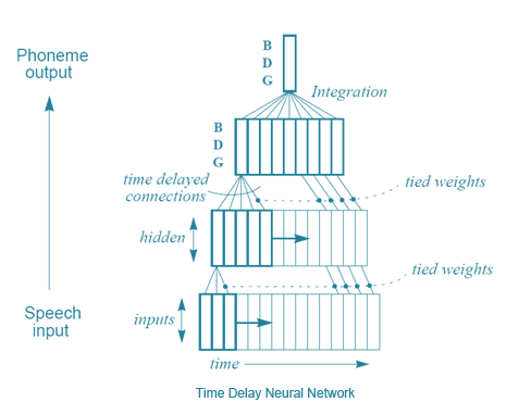
In a sense, this is quite similar to what CNNs do - instead of looking at the whole input at once, each unit looks at just a subset of the input at a time and does the same computation for each small subset. The main difference here is that there is no idea of time in a CNN, and the ‘window’ of input for each neuron is always moved across the whole input image to compute a result, whereas in a TDNN there actually is sequential input and output of data. Fun fact: according to Hinton, the idea of TDNNs is what inspired LeCun to develop convolutional neural nets. But, funnily enough CNNs became essential for image processing, whereas in speech recognition TDNNs have been surpassed to another approach - recurrent neural nets (RNNs). See, all the networks that have been discussed so far have been feedforward networks, meaning that the output of neurons in a given layer acts as input to only neurons in a next layer. But, it does not have to be so - there is nothing prohibiting us brave computer scientists from connecting output of the last layer act as an input to the first layer, or just connecting the output of a neuron to itself. By having the output of the network ‘loop’ back into the network, the problem of giving the network memory as to past inputs is solved so elegantly!
Again, those seeking greater insight into the distinctions between different neural nets would do well to just go back to the actual papers. Here is a nice summation of why RNNs are cooler than TDNNs for sequential data: "A recurrent network has cycles in its graph that allow it to store information about past inputs for an amount of time that is not fixed a priori but rather depends on its weights and on the input data. The type of recurrent networks considered here can be used either for sequence recognition production or prediction. Units are not clamped and we are not interested in convergence to a fixed point. Instead the recurrent network is used to transform an input sequence eg speech spectra into an output sequence, eg degrees, of evidence for phonemes. The main advantage of such recurrent networks is that the relevant past context can be represented in the activity of the hidden units and then used to compute the output at each time step. In theory the network can learn how to extract the relevant context information from the input sequence. In contrast, in network with time delays such as TDNNs the designer of the network must decide a priori by the choice of delay connections which part of the past input sequence should be used to predict the next output. According to the terminology introduced in [] the memory is static in the case of TDNNs but it is adaptive in the case of recurrent networks."
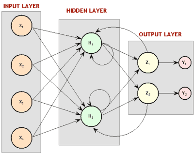
Well, it’s not quite so simple. Notice the problem - if backpropagation relies on ‘propagating’ the error from the output layer backward, how do things work if the first layer connects back to the output layer? The error would go ahead and propagate from the first layer back to the output layer, and could just keep looping through the network, infinitely. The solution, independently derived by multiple groups, is backpropagation through time. Basically, the idea is to ‘unroll’ the recurrent neural network by treating each loop through the neural network as an input to another neural network, and looping only a limited number of times.

This fairly simple idea actually worked - it was possible to train recurrent neural nets. And indeed, multiple people explored the application of RNNs to speech recognition. But, here is a twist you should now be able to predict: this approach did not work very well. To find out why, let’s meet another modern giant of Deep Learning: Yoshua Bengio. Starting work on speech recognition with neural nets around 1986, he co-wrote many papers on using ANNs and RNNs for speech recognition, and ended up working at the AT&T Bell Labs on the problem just as Yann LeCun was working with CNNs there. In fact, in 1995 they co-wrote the summary paper “Convolutional Networks for Images, Speech, and Time-Series”38, the first of many collaborations among them. But, before then Bengio wrote the 1993 “A Connectionist Approach to Speech Recognition”39. Here, he summarized the general failure of effectively teaching RNNs:
“Although recurrent networks can in many instances outperform static networks, they appear more difficult to train optimally. Our experiments tended to indicate that their parameters settle in a suboptimal solution which takes into account short term dependencies but not long term dependencies. For example in experiments described in (ctation) we found that simple duration constraints on phonemes had not at all been captured by the recurrent network. … Although this is a negative result, a better understanding of this problem could help in designing alternative systems for learning to map input sequences to output sequences with long term dependencies eg for learning finite state machines, grammars, and other language related tasks. Since gradient based methods appear inadequate for this kind of problem we want to consider alternative optimization methods that give acceptable results even when the criterion function is not smooth.”
Neural Nets Start to Speak
Speaking of Bengio, his contributions with respect to neural nets go well beyond this work with CNNs and RNNs. In particular, this history would not be complete without covering his seminal paper 2003 “A Neural Probabilistic Language Model”. As the title implies, this work had to do with using neural nets to do language modeling – a fundamental task in the field of Natural Language Processing, which boils down to predicting what seeing some number of words and predicting what words come next (essentially, what autocomplete does). The task has by then been studied for a long time, with the classical approaches essentially being to count how often individual words and varios word combiations (otherwise known as n-grams) happen in a bunch of text, and then using these counts to estimate the probability for any given word being the one to come next:
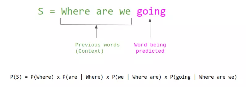
While this approach was highly succesful, it was also inherently limited, since it required seeing a word or a combination of words to predict where it would occur, and human language has an huge number of words which have exponentially many combinations. In contrast, us humans don’t only reason about language in terms of what we have seen but also what we know about each word’s meaning; if we have only seen “I have a pet dog” and then learn that there exists such as word as “cat” that is also a common pet, we would have no trouble imagining that “I have a pet cat” as something that someone is likely to say.
So, how do we get computers to understand how similar different words are? After all, the meaning of words are quite subtle, and something simple like comparing words’ definitions in terms of what words are in them is therefore not likely to work well. Well, it turns out that the subtlety of meaning can nicely be captured in a format that also easily allows for evaluating similarity: lists of numbers. Just as any (x,y) point in a 2D space has a known distance from any other point in that space, so does any point in a 100D space have known distances from all other points, and it could be said that closer points are more similar and farther points are less similar. Therefore, if we could map every word to an appropriate point in a many-dimensional space, such that similar words are mapped to nearby points, that should be quite useful for language modeling. Hinrich Schütze introduced this idea in his 1993 papers “Word Space”, in which he showed how to compute “Word Vectors” with matrix processing over counts of phrase co-occurences, resulting in the ability to find the most similar words for any given query word:
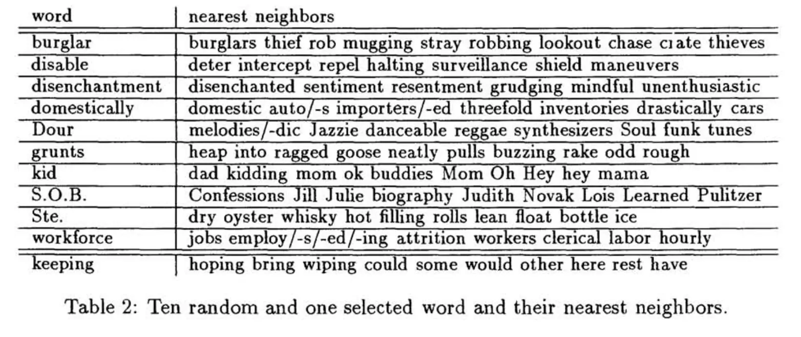
So, where do neural nets enter this picture? Well, there are many ways one could get word vectors, and the above paper’s approach was just one. What if instead, you used the word vectors as inputs to a neural net that was optimized to correctly do language modeling? And then both the vectors associated with the word’s and the overall neural net’s ability to correctly do language modeling can be jointly optimized using backpropagation from the appropriate error function. And that’s where we get back to A Neural Probabilistic Language Model, since that’s what the paper essentially describes.
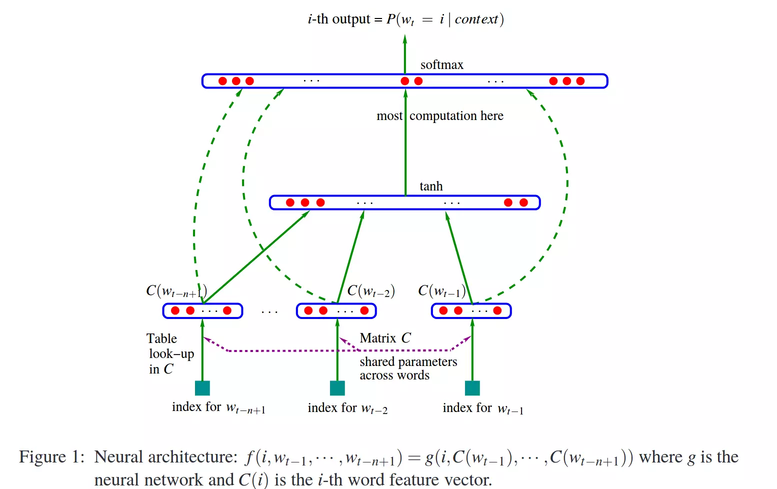
This is now a hugely cited work, but as with the other things we’ve seen above, it took some time for the usefulness of word vectors and neural nets for language modeling to be appreciated. And we shall see why next…
A New Winter Dawns
Back to the 90s – there was a problem. A big problem. And the problem, basically, was what so recently was a huge advance: backpropagation. See, convolutional neural nets were important in part because backpropagation just did not work well for normal neural nets with many layers. And that’s the real key to deep-learning - having many layers, in today’s systems as many as 20 or more. But already by the late 1980’s, it was known that deep neural nets trained with backpropagation just did not work very well, and particularly did not work as well as nets with fewer layers. The reason, in basic terms, is that backpropagation relies on finding the error at the output layer and successively splitting up blame for it for prior layers. Well, with many layers this calculus-based splitting of blame ends up with either huge or tiny numbers and the resulting neural net just does not work very well - the ‘vanishing or exploding gradient problem’. Jurgen Schmidhuber, another Deep Learning luminary, summarizes the more formal explanation well40:
“A diploma thesis (Hochreiter, 1991) represented a milestone of explicit DL research. As mentioned in Sec. 5.6, by the late 1980s, experiments had indicated that traditional deep feedforward or recurrent networks are hard to train by backpropagation (BP) (Sec. 5.5). Hochreiter’s work formally identified a major reason: Typical deep NNs suffer from the now famous problem of vanishing or exploding gradients. With standard activation functions (Sec. 1), cumulative backpropagated error signals (Sec. 5.5.1) either shrink rapidly, or grow out of bounds. In fact, they decay exponentially in the number of layers or CAP depth (Sec. 3), or they explode. “
Backpropagation through time is essentially equivalent to a neural net with a whole lot of layers, so RNNs were particularly difficult to train with Backpropagation. Both Sepp Hochreiter, advised by Schmidhuber, and Yoshua Bengio published papers on the inability of learning long-term information due to limitations of backpropagation 4142. The analysis of the problem did reveal a solution - Schmidhuber and Hochreiter introduced a very important concept in 1997 that essentially solved the problem of how to train recurrent neural nets, much as CNNs did for feedforward neural nets - Long Short Term Memory (LSTM)43. In simple terms, as with CNNs the LTSM breakthrough ended up being a small alteration to the normal neural net model 40:
“The basic LSTM idea is very simple. Some of the units are called Constant Error Carousels (CECs). Each CEC uses as an activation function f, the identity function, and has a connection to itself with fixed weight of 1.0. Due to f’s constant derivative of 1.0, errors backpropagated through a CEC cannot vanish or explode (Sec. 5.9) but stay as they are (unless they “flow out” of the CEC to other, typically adaptive parts of the NN). CECs are connected to several nonlinear adaptive units (some with multiplicative activation functions) needed for learning nonlinear behavior. Weight changes of these units often profit from error signals propagated far back in time through CECs. CECs are the main reason why LSTM nets can learn to discover the importance of (and memorize) events that happened thousands of discrete time steps ago, while previous RNNs already failed in case of minimal time lags of 10 steps.”
But, this did little to fix the larger perception problem that neural nets were janky and did not work very well. They were seen as a hassle to work with - the computers were not fast enough, the algorithms were not smart enough, and people were not happy. So, around the mid 90s, a new AI Winter for neural nets began to emerge - the community once again lost faith in them. A new method called Support Vector Machines, which in the very simplest terms could be described as a mathematically optimal way of training an equivalent to a two layer neural net, was developed and started to be seen as superior to the difficult to work with neural nets. In fact, the 1995 “Comparison of Learning Algorithms For Handwritten Digit Recognition”44 by LeCun et al. found that this new approach worked better or the same as all but the best designed neural nets:
“The [support vector machine] classifier has excellent accuracy, which is most remarkable, because unlike the other high performance classifiers, it does not include a priori knowledge about the problem. In fact, this classifier would do just as well if the image pixels were permuted with a fixed mapping. It is still much slower and memory hungry than the convolutional nets. However, improvements are expected as the technique is relatively new.”
Other new methods, notably Random Forests, also proved to be very effective and with lovely mathematical theory behind them. So, despite the fact that CNNs consistently had state of the art performance, enthusiasm for neural nets dissipated and the machine learning community at large once again disavowed them. Winter was back. But worry not, for next we shall see how a small group of researchers persevered in this research climate and ultimately made Deep Learning what it is today.
“Ask anyone in machine learning what kept neural network research alive and they will probably mention one or all of these three names: Geoffrey Hinton, fellow Canadian Yoshua Bengio and Yann LeCun, of Facebook and New York University.”45
Part 3: Deep Learning (2000s-2010s)
In this last part of our history, we will get to the end of our story and see how deep learning emerged from the slump neural nets found themselves in by the late 90s, and the amazing state of the art results it has achieved since.
The Funding of More Layers
With the ascent of Support Vector Machines and the failure of backpropagation, the early 2000s were a dark time for neural net research. LeCun and Hinton variously mention how in this period their papers or the papers of their students were routinely rejected from being published due to their subject being Neural Nets. Certainly research in Machine Learning and AI was still very active, and other people were also still working with neural nets, but citation counts from the time make it clear that the excitement had leveled off, even if it did not completely evaporate. Still, Hinton, Bengio, and Lecun in particular persevered in their belief neural nets merit research.
And they found a strong ally outside the research realm: The Canadian government. Funding from the Canadian Institute for Advanced Research (CIFAR), which encourages basic research without direct application, was what motivated Hinton to move to Canada in 1987, and funded his work afterward. But, the funding was ended in the mid 90s just as sentiment towards neural nets was becoming negative again. Rather than relenting and switching his focus, Hinton fought to continue work on neural nets, and managed to secure more funding from CIFAR as told well in this exemplary piece45:
“But in 2004, Hinton asked to lead a new program on neural computation. The mainstream machine learning community could not have been less interested in neural nets.
“It was the worst possible time,” says Bengio, a professor at the Université de Montréal and co-director of the CIFAR program since it was renewed last year. “Everyone else was doing something different. Somehow, Geoff convinced them.”
“We should give (CIFAR) a lot of credit for making that gamble.”
CIFAR “had a huge impact in forming a community around deep learning,” adds LeCun, the CIFAR program’s other co-director. “We were outcast a little bit in the broader machine learning community: we couldn’t get our papers published. This gave us a place where we could exchange ideas.””
The funding was modest, but sufficient to enable a small group of researchers to keep working on the topic. As Hinton tells it, they hatched a conspiracy: “rebrand” the frowned-upon field of neural nets with the moniker “deep learning” 45. Then, what every researcher must dream of actually happened: Hinton, Simon Osindero, and Yee-Whye Teh published a paper in 2006 that was seen as a breakthrough, a breakthrough significant enough to rekindle interest in neural nets: A fast learning algorithm for deep belief nets46. Though, as we’ll see, the approaches used in the paper have been superceded by newer work, the movement that is ‘deep learning’ can be said to have started precisely with this paper. But, more important than the name was the idea - that neural networks with many layers really could be trained well, if the weights are initialized in a clever way rather than randomly. Hinton once expressed the need for such an advance at the time:
“Historically, this was very important in overcoming the belief that these deep neural networks were no good and could never be trained. And that was a very strong belief. A friend of mine sent a paper to ICML [International Conference on Machine Learning], not that long ago, and the referee said it should not accepted by ICML, because it was about neural networks and it was not appropriate for ICML. In fact if you look at ICML last year, there were no papers with ‘neural’ in the title accepted, so ICML should not accept papers about neural networks. That was only a few years ago. And one of the IEEE journals actually had an official policy of [not accepting your papers]. So, it was a strong belief.”
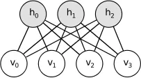
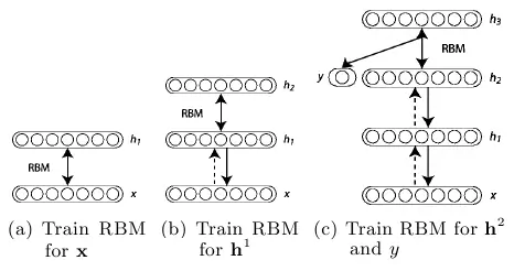
So what was the clever way of initializing weights? The basic idea is to train each layer one by one with unsupervised training, which starts off the weights much better than just giving them random values, and then finishing with a round of supervised learning just as is normal for neural nets. Each layer starts out as a Restricted Boltzmann Machine (RBM), which is just a Boltzmann Machine without connections between hidden and visible units as illustrated above, and is taught a generative model of data in an unsupervised fashion. It turns out that this form of Boltzmann machine can be trained in an efficient manner introduced by Hinton in the 2002 “Training Products of Experts by Minimizing Contrastive Divergence”47. Basically, this algorithm maximizes something other than the probability of the units generating the training data, which allows for a nice approximation and turns out to still work well. So, using this method, the algorithm is as such:
- Train an RBM on the training data using contrastive-divergence. This is the first layer of the belief net.
- Generate the hidden values of the trained RBM for the data, and train another RBM using those hidden values. This is the second layer - ‘stack’ it on top of the first and keep weights in just one direction to form a belief net.
- Keep doing step 2 for as many layers as are desired for the belief net.
- If classification is desired, add a small set of hidden units that correspond to the classification labels and do a variation on the wake-sleep algorithm to ‘fine-tune’ the weights. Such combinations of unsupervised and supervised learning are often called semi-supervised learning.
The paper concluded by showing that deep belief networks (DBNs) had state of the art performance on the standard MNIST character recognition dataset, significantly outperforming normal neural nets with only a few layers. Yoshua Bengio et al. followed up on this work in 2007 with “Greedy Layer-Wise Training of Deep Networks”48, in which they present a strong argument that deep machine learning methods (that is, methods with many processing steps, or equivalently with hierarchical feature representations of the data) are more efficient for difficult problems than shallow methods (which two-layer ANNs or support vector machines are examples of).
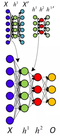
They also present reasons for why the addition of unsupervised pre-training works, and conclude that this not only initializes the weights in a more optimal way, but perhaps more importantly leads to more useful learned representations of the data. In fact, using RBMs is not that important - unsupervised pre-training of normal neural net layers using backpropagation with plain Autoencoders layers proved to also work well. Likewise, at the same time another approach called Sparse Coding also showed that unsupervised feature learning was a powerful approach for improving supervised learning performance.
So, the key really was having many layers of computing units so that good high-level representation of data could be learned - in complete disagreement with the traditional approach of hand-designing some nice feature extraction steps and only then doing learning using those features. Hinton and Bengio’s work had empirically demonstrated that fact, but more importantly, showed the premise that deep neural nets could not be trained well to be false. This, LeCun had already demonstrated with CNNs throughout the 90s, but neural nets still went out of favor. Bengio, in collaboration with Yann LeCun, reiterated this on “Scaling Algorithms Towards AI”49:
“Until recently, many believed that training deep architectures was too difficult an optimization problem. However, at least two different approaches have worked well in training such architectures: simple gradient descent applied to convolutional networks [LeCun et al., 1989, LeCun et al., 1998] (for signals and images), and more recently, layer-by-layer unsupervised learning followed by gradient descent [Hinton et al., 2006, Bengio et al., 2007, Ranzato et al., 2006]. Research on deep architectures is in its infancy, and better learning algorithms for deep architectures remain to be discovered. Taking a larger perspective on the objective of discovering learning principles that can lead to AI has been a guiding perspective of this work. We hope to have helped inspire others to seek a solution to the problem of scaling machine learning towards AI.”
And inspire they did. Or at least, they started; though deep learning had not yet gained the tsumani momentum that it has today, the wave had unmistakably begun. Still, the results at that point were not that impressive - most of the demonstrated performance in the papers up to this point was for the MNIST dataset, a classic machine learning task that had been the standard benchmark for algorithms for about a decade. Hinton’s 2006 publication demonstrated a very impressive error rate of only 1.25% on the test set, but SVMs had already gotten an error rate of 1.4%, and even simple algorithms could get error rates in the low single digits. And, as was pointed out in the paper, Yann LeCun already demonstrated error rates of 0.95% in 1998 using CNNs in the paper “Gradient-based learning applied to document recognition”.
So, doing well on MNIST was not necessarily that big a deal. Aware of this and confident that it was time for deep learning to take the stage, Hinton and two of his graduate students, Abdel-rahman Mohamed and George Dahl, demonstrated their effectiveness at a far more challenging AI task: Speech Recognition50. Using DBNs, the two students and Hinton managed to improve on a decade-old performance record on a standard speech recognition dataset. This was an impressive achievement, but in retrospect seems like only a hint at what was coming – in short, many more broken records.
The Development of Big Data
So, algorithmic advancements were certainly made and led to increasing excitement about neural nets. But, this alone did not overcome the limitations of neural nets seen in the 90s. After all, to train a neural net you don’t only need the optimization algorithm, you also need another crucial ingredient: the data. As we’ve covered long ago near the start of this piece, neural nets are often trained via supervised training from labeled examples, and so to apply them to any given problem requires having this data.
But, to tackle difficult tasks neural nets need lots of such data, getting large datasets is not trivial. While it may not seem as conceptually difficult as coming up with clever algorithms, it’s still a lot of work, and having the insight to decide on the right inputs and outputs to enable new research it also important. So, it’s crucial not to overlook this topic or take it for granted. We’ve already mentioned The MNIST database of handwritten digits (“a classic machine learning task that had been the standard benchmark for algorithms for about a decade”), which was made by modifying data first released by the National Institute of Standards and Technology in 1995. Next, we’ll look at the datasets that emerged in the 2000s and were crucial to the development of deep learning.
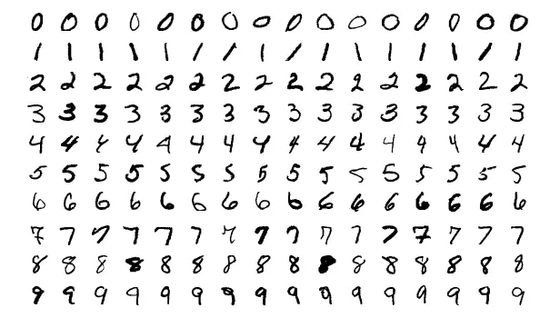
But, there is only so much you can do with a dataset of hand-written digits. Computer Vision aims at enabling machines to understand images in ways analogous to humans, which of course includes recognizing what objects are present in a given image. So, in the 2000s researchers set out to create datasets that could be used to work on this problem. Starting in 2005, there was the annual The PASCAL Visual Object Classes (VOC) Challenge. Then there were also Caltech 101 and Caltech 256 datasets, likewise influential for Computer Vision research. But for our topic of deep learning, there is undoubtedly a most important development to focus on: ImageNet.
As covered well in Quartz’s The data that transformed AI research — and possibly the world, Professor Fei-Fei Li’s idea of creating a dataset containing images for most of the concepts in the massive WordNet database (which is like a giant dictionary of english words grouped by their meanings) required creating a dataset of unprecedented size. Fortunately, soon after the idea came about so did the option to crowdsource (split the work of labeling data to many people via the internet), and the project could go ahead. Still, it took years of work before Li and her students and collaborators released their dataset and a paper in 2009. By then, the dataset had 3.2 million images for 5247 concepts, still a long way away from the final goal of 50 million images but also orders of magnitude larger than the scale of prior datasets.

Still, it was not immediately apparent to the Computer Vision community that this dataset would indeed enable major advancements. After all, and learning to categorize so many different types of objects from so large a set of images was not yet attempted that the algorithms of that day. Even when the dataset was paired down for the ImageNet Large Scale Visual Recognition Challenge (which had just 1000 types of objects and only 150,000 images), the first year’s winning entry could not pick the right category with 5 guesses for 30% of the test dataset. So, it was a hard problem, and therefore also a good challenge with which to demonstrate the potential of neural nets. But, it will take several more years and the last piece of the deep learning puzzle for us to get to that…
The Importance of Brute Force
The algorithmic advances and new datasets described above were undoubtedly important to the emergence of deep learning, but there was another essential component that had emerged in the decade since the 1990s: pure computational power. Following Moore’s law, computers got dozens of times faster since the slow days of the 90s, making learning with large datasets and many layers much more tractable. But even this was not enough - CPUs were starting to hit a ceiling in terms of speed growth, and computer power was starting to increase mainly through weakly parallel computations with several CPUs. To learn the millions of weights typical in deep models, the limitations of weak CPU parallelism had to be left behind and replaced with the massively parallel computing powers of GPUs. Realizing this is, in part, how Abdel-rahman Mohamed, George Dahl, and Geoff Hinton accomplished their record breaking speech recognition performance51:
“Inspired by one of Hinton’s lectures on deep neural networks, Mohamed began applying them to speech - but deep neural networks required too much computing power for conventional computers – so Hinton and Mohamed enlisted Dahl. A student in Hinton’s lab, Dahl had discovered how to train and simulate neural networks efficiently using the same high-end graphics cards which make vivid computer games feasible on personal computers.
They applied the same method to the problem of recognizing fragments of phonemes in very short windows of speech,” said Hinton. “They got significantly better results than previous methods on a standard three-hour benchmark.””
It’s hard to say just how much faster using GPUs over CPUs was in this case, but the paper “Large-scale Deep Unsupervised Learning using Graphics Processors”52 of the same year suggests a number: 70 times faster. Yes, 70 times - reducing weeks of work into days, even a single day. The authors, who had previously developed Sparse Coding, included the prolific Machine Learning researcher Andrew Ng, who increasingly realized that making use of lots of training data and of fast computation had been greatly undervalued by researchers in favor of incremental changes in learning algorithms. This idea was strongly supported by 2010’s “Deep Big Simple Neural Nets Excel on Handwritten Digit Recognition”53 (notably co-written by J. Schmidhuber, one of the inventors of the recurrent LTSM networks), which showed a whopping %0.35 error rate could be achieved on the MNIST dataset without anything more special than really big neural nets, a lot of variations on the input, and efficient GPU implementations of backpropagation. These ideas had existed for decades, so although it could not be said that algorithmic advancements did not matter, this result did strongly support the notion that the brute force approach of big training sets and fast parallelized computations were also crucial.
Dahl and Mohamed’s use of a GPU to get record breaking results was an early and relatively modest success, but it was sufficient to incite excitement and for the two to be invited to intern at Microsoft Research45. Here, they would have the benefit from another trend in computing that had emerged by then: Big Data. That loosest of terms, which in the context of machine learning is easy to understand - lots of training data. And lots of training data is important, because without it neural nets still did not do great - they tended to overfit (perfectly work on the training data, but not generalize to new test data). This makes sense - the complexity of what large neural nets can compute is such that a lot of data is needed to avoid them learning every little unimportant aspect of the training set - but was a major challenge for researchers in the past. So now, the computing and data gathering powers of large companies proved invaluable. The two students handily proved the power of deep learning during their three month internship, and Microsoft Research has been at the forefront of deep learning speech recognition ever since.
Microsoft was not the only BigCompany to recognize the power of deep learning (though it was handily the first). Navdeep Jaitly, another student of Hinton’s, went off to a summer internship at Google in 2011. There, he worked on Google’s speech recognition, and showed their existing setup could be much improved by incorporating deep learning. The revised approach soon powered Android’s speech recognition, replacing much of Google’s carefully crafted prior solution 45.
Besides the impressive effects of humble PhD interns on these gigantic companies’ products, what is notable here is that both companies were making use of the same ideas - ideas that were out in the open for anyone to work with. And in fact, the work by Microsoft and Google, as well as IBM and Hinton’s lab, resulted in the impressively titled “Deep Neural Networks for Acoustic Modeling in Speech Recognition: The Shared Views of Four Research Groups”54 in 2012. Four research groups - three from companies that could certainly benefit from a briefcase full of patents on the emerging wonder technology of deep learning, and the university research group that popularized that technology - working together and publishing their results to the broader research community. If there was ever an ideal scenario for industry adopting an idea from research, this seems like it.
Not to say the companies were doing this for charity. This was the beginning of all of them exploring how to commercialize the technology, and most of all Google. But it was perhaps not Hinton, but Andrew Ng who incited the company to become likely the world’s biggest commercial adopter and proponent of the technology. In 2011, Ng incidentally met with the legendary Googler Jeff Dean while visiting the company, and chatted about his efforts to train neural nets with Google’s fantastic computational resources. This intrigued Dean, and together with Ng they formed Google Brain - an effort to build truly giant neural nets and explore what they could do. The work resulted in unsupervised neural net learning of an unprecedented scale - 16,000 CPU cores powering the learning of a whopping 1 billion weights (for comparison, Hinton’s breakthrough 2006 DBN had about 1 million weights). The neural net was trained on Youtube videos, entirely without labels, and learned to recognize the most common objects in those videos - leading of course to the internet’s collective glee over the net’s discovery of cats:
Cute as that was, it was also useful. As they reported in a regularly published paper, the features learned by the model could be used for record setting performance on a standard computer vision benchmark55. With that, Google’s internal tools for training massive neural nets were born, and they have only continued to evolve since. The wave of deep learning research that began in 2006 had now undeniably made it into industry.
The Deep Learning Equation
While deep learning was making it into industry, the research community was hardly keeping still. The discovery that efficient use of GPUs and computing power in general was so important made people examine long-held assumptions and ask questions that should have perhaps been asked long ago - namely, why exactly does backpropagation not work well? The insight to ask why the old approaches did not work, rather than why the new approaches did, led Xavier Glort and Yoshua Bengio to write “Understanding the difficulty of training deep feedforward neural networks” in 201056. In it, they discussed two very meaningful findings:
- The particular non-linear activation function chosen for neurons in a neural net makes a big impact on performance, and the one often used by default is not a good choice.
- It was not so much choosing random weights that was problematic, as choosing random weights without consideration for which layer the weights are for. The old vanishing gradient problem happens, basically, because backpropagation involves a sequence of multiplications that invariably result in smaller derivatives for earlier layers. That is, unless weights are chosen with difference scales according to the layer they are in - making this simple change results in significant improvements.
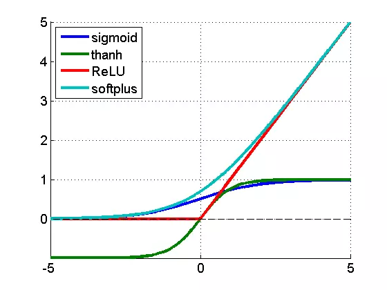
The second point is quite clear, but the first opens the question: ‘what, then, is the best activation function’? Three different groups explored the question (a group with LeCun, with “What is the best multi-stage architecture for object recognition?”57, a group with Hinton, in “Rectified linear units improve restricted boltzmann machines”58, and a group with Bengio -“Deep Sparse Rectifier Neural Networks”59), and they all found the same surprising answer: the very much non-differentiable and very simple function f(x)=max(0,x) tends to be the best. Surprising, because the function is kind of weird - it is not strictly differentiable, or rather is not differentiable precisely at zero, so on paper as far as math goes it looks pretty ugly. But, clearly the zero case is a pretty small mathematical quibble - a bigger question is why such a simple function, with constant derivatives on either side of 0, is so good. The answer is not precisely known, but a few ideas seem pretty well established:
- Rectified activation leads to sparse representations, meaning not many neurons actually end up needing to output non-zero values for any given input. In the years leading up to this point sparsity was shown to be beneficial for deep learning, both because it represents information in a more robust manner and because it leads to significant computational efficiency (if most of your neurons are outputting zero, you can in effect ignore most of them and compute things much faster). Incidentally, researchers in computational neuroscience first introduced the importance of sparse computation in the context of the brain’s visual system, a decade before it was explored in the context of machine learning.
- The simplicity of the function, and its derivatives, makes it much faster to work with than the exponential sigmoid or the trigonometric tanh. As with the use of GPUs, this turns out to not just be a small boost but really important for being able to scale neural nets to the point where they perform well on challenging problems.
- A later analysis titled “Rectifier Nonlinearities Improve Neural Network Acoustic Models”60, co-written by Andrew Ng, also showed the constant 0 or 1 derivative of the ReLU not too detrimental to learning. In fact, it helps avoid the vanishing gradient problem that was the bane of backpropagation. Furthermore, beside producing more sparse representations, it also produces more distributed representations - meaning is derived from the combination of multiple values of different neurons, rather than being localized to individual neurons.
At this point, with all these discoveries since 2006, it had become clear that unsupervised pre-training is not essential to deep learning. It was helpful, no doubt, but it was also shown that in some cases well-done, purely supervised training (with the correct starting weight scales and activation function) could outperform training that included the unsupervised step. So, why indeed, did purely supervised learning with backpropagation not work well in the past? Geoffrey Hinton summarized the findings up to today in these four points:
- Our labeled datasets were thousands of times too small.
- Our computers were millions of times too slow.
- We initialized the weights in a stupid way.
- We used the wrong type of non-linearity.
So here we are. Deep learning. The culmination of decades of research, all leading to this:
Deep Learning =
Lots of training data + Parallel Computation + Scalable, smart algorithms

Not to say all there was to figure out was figured out by this point. Far from it. What had been figured out is exactly the opposite: that peoples’ intuition was often wrong, and in particular unquestioned decisions and assumptions were often very unfounded. Asking simple questions, trying simple things - these had the power to greatly improve state of the art techniques. And precisely that has been happening, with many more ideas and approaches being explored and shared in deep learning since. An example: “Improving neural networks by preventing co-adaptation of feature detectors”61 by G. E. Hinton et al. The idea is very simple: to prevent overfitting, randomly pretend some neurons are not there while training. This straightforward idea - called Dropout - is a very efficient means of implementing the hugely powerful approach of ensemble learning, which just means learning in many different ways from the training data. Random Forests, a dominating technique in machine learning to this day, is chiefly effective due to being a form of ensemble learning. Training many different neural nets is possible but is far too computationally expensive, yet this simple idea in essence achieves the same thing and indeed significantly improves performance.
Still, having all these research discoveries since 2006 is not what made the computer vision or other research communities again respect neural nets. What did do it was something somewhat less noble: completely destroying non-deep learning methods on a modern competitive benchmark. Geoffrey Hinton enlisted two of his Dropout co-writers, Alex Krizhevsky and Ilya Sutskever, to apply the ideas discovered to create an entry to the ImageNet Large Scale Visual Recognition Challenge (ILSVRC)-2012 computer vision competition. To me, it is very striking to now understand that their work, described in “ImageNet Classification with deep convolutional neural networks”62, is the combination of very old concepts (a CNN with pooling and convolution layers, variations on the input data) with several new key insight (very efficient GPU implementation, ReLU neurons, dropout), and that this, precisely this, is what modern deep learning is.
So, how did they do? Far, far better than the next closest entry: their error rate was %15.3, whereas the second closest was %26.2. This, the first and only CNN entry in that competition, was an undisputed sign that CNNs, and deep learning in general, had to be taken seriously for computer vision. Now, almost all entries to the competition are CNNs - a neural net model Yann LeCun was working with since 1989. And, remember LSTM recurrent neural nets, devised in the 90s by Sepp Hochreiter and Jürgen Schmidhuber to solve the backpropagation problem? Those, too, are now state of the art for sequential tasks such as speech processing.
This was the turning point. A mounting wave of excitement about possible progress has culminated in undeniable achievements that far surpassed what other known techniques could manage. The tsunami metaphor that we started with in part 1, this is where it began, and it has been growing and intensifying to this day. Deep learning is here, and no winter is in sight.
Epilogue: The Decade of Deep Learning
If this were a movie, the 2012 ImageNet competition would likely have been the climax, and now we would have a progression of text describing ‘where are they now’. Yann LeCun - Facebook. Geoffrey Hinton - Google. Andrew Ng - Coursera, Google, Baidu, and more. Bengio, Schmidhuber, and Li actually still in academia but with their own industry affiliations too, and presumably with many more citations and/or grad students63 (and, the many more who contributed to the emergence of Deep Learning . Though the ideas and achievements of deep learning are definitely exciting, while writing this I was inevitably also moved that these people, who worked in this field for decades (even as most abandoned it), are now rich, successful, and most of all better situated to do research than ever. All these peoples’ ideas are still very much out in the open, and in fact basically all these companies are open sourcing their deep learning frameworks, like some sort of utopian vision of industry-led research. What a story.
Since 2012, it’s fair to say Deep Learning has revolutionized much of AI as a field. As we read at the start of all this, “2015 seems like the year when the full force of the tsunami hit the major Natural Language Processing (NLP) conferences.” And so it was with Computer Vision, Robotics, Audio Processing, AI for Medicine, and so much more. To summarize all the ground breaking developments in this period would take its own lengthy sub-history, and has already been done nicely in the blog post “The Decade of Deep Learning”. Suffice it today, progress since 2012 was swift and ongoing, and has seen all the applications of neural nets we have seen so far (to reinforcement learning, language modeling, image classification, and much more) extended to leverage Deep Learning resulting in ground breaking accomplishments.
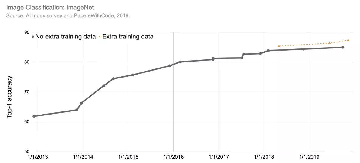
With such progress came much excitement, and the field of AI rapidly grew:
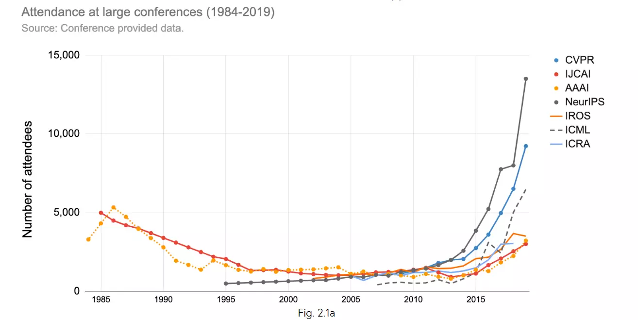
And now here were at 2020. AI as a field is huge and still moving fast, but many of the low-hanging fruit with respect to tackling AI problems with Deep Learning have been plucked, and we are increasingly in a time expanding outwards in terms of varied applications of neural nets and Deep Learning64. And for good reason: Deep Learning still works best only when there is a huge dataset of input-output examples to learn from, which is not true for many problems in AI, and has other major limitations (interpretability, verifiability, and more). Although this is where this brief history, the history of neural nets is very much still being written, and shall be for some time. Let us hope this powerful technology continues to blossom, and is used primarily to further human well-being and progress well into the future.
Citation
This piece is an updated and expanded version of blog posts originally released in 2015 on www.andreykurenkov.com. Please cite this version.
For attribution in academic contexts or books, please cite this work as
Andrey Kurenkov, “A Brief History of Neural Nets and Deep Learning”, Skynet Today, 2020.
BibTeX citation:
@article{kurenkov2020briefhistory,
author = {Kurenkov, Andrey},
title = {A Brief History of Neural Nets and Deep Learning},
journal = {Skynet Today},
year = {2020},
howpublished = {\url{https://skynettoday.com/overviews/neural-net-history } },
}
-
Christopher D. Manning. (2015). Computational Linguistics and Deep Learning Computational Linguistics, 41(4), 701–707. ↩
-
F. Rosenblatt. The perceptron, a perceiving and recognizing automaton Project Para. Cornell Aeronautical Laboratory, 1957. ↩
-
W. S. McCulloch and W. Pitts. A logical calculus of the ideas immanent in nervous activity. The bulletin of mathematical biophysics, 5(4):115–133, 1943. ↩
-
The organization of behavior: A neuropsychological theory. D. O. Hebb. John Wiley And Sons, Inc., New York, 1949 ↩
-
B. Widrow et al. Adaptive ”Adaline” neuron using chemical ”memistors”. Number Technical Report 1553-2. Stanford Electron. Labs., Stanford, CA, October 1960. ↩
-
“New Navy Device Learns By Doing”, New York Times, July 8, 1958. ↩
-
Perceptrons. An Introduction to Computational Geometry. MARVIN MINSKY and SEYMOUR PAPERT. M.I.T. Press, Cambridge, Mass., 1969. ↩
-
Minsky, M. (1952). A neural-analogue calculator based upon a probability model of reinforcement. Harvard University Pychological Laboratories internal report. ↩
-
Linnainmaa, S. (1970). The representation of the cumulative rounding error of an algorithm as a Taylor expansion of the local rounding errors. Master’s thesis, Univ. Helsinki. ↩
-
P. Werbos. Beyond Regression: New Tools for Prediction and Analysis in the Behavioral Sciences. PhD thesis, Harvard University, Cambridge, MA, 1974. ↩
-
Werbos, P.J. (2006). Backwards differentiation in AD and neural nets: Past links and new opportunities. In Automatic Differentiation: Applications, Theory, and Implementations, pages 15-34. Springer. ↩
-
Rumelhart, D. E., Hinton, G. E., and Williams, R. J. (1986). Learning representations by back-propagating errors. Nature, 323, 533–536. ↩
-
Widrow, B., & Lehr, M. (1990). 30 years of adaptive neural networks: perceptron, madaline, and backpropagation. Proceedings of the IEEE, 78(9), 1415-1442. ↩
-
D. E. Rumelhart, G. E. Hinton, and R. J. Williams. 1986. Learning internal representations by error propagation. In Parallel distributed processing: explorations in the microstructure of cognition, vol. 1, David E. Rumelhart, James L. McClelland, and CORPORATE PDP Research Group (Eds.). MIT Press, Cambridge, MA, USA 318-362 ↩
-
Kurt Hornik, Maxwell Stinchcombe, Halbert White, Multilayer feedforward networks are universal approximators, Neural Networks, Volume 2, Issue 5, 1989, Pages 359-366, ISSN 0893-6080, http://dx.doi.org/10.1016/0893-6080(89)90020-8. ↩
-
LeCun, Y; Boser, B; Denker, J; Henderson, D; Howard, R; Hubbard, W; Jackel, L, “Backpropagation Applied to Handwritten Zip Code Recognition,” in Neural Computation , vol.1, no.4, pp.541-551, Dec. 1989 89 ↩
-
D. E. Rumelhart, G. E. Hinton, and R. J. Williams. 1986. Learning internal representations by error propagation. In Parallel distributed processing: explorations in the microstructure of cognition, vol. 1, David E. Rumelhart, James L. McClelland, and CORPORATE PDP Research Group (Eds.). MIT Press, Cambridge, MA, USA 318-362 ↩ ↩2
-
Fukushima, K. (1980), ‘Neocognitron: A Self-Organizing Neural Network Model for a Mechanism of Pattern Recognition Unaffected by Shift in Position’, Biological Cybernetics 36 , 193–202 . ↩
-
Gregory Piatetsky, ‘KDnuggets Exclusive: Interview with Yann LeCun, Deep Learning Expert, Director of Facebook AI Lab’ Feb 20, 2014. http://www.kdnuggets.com/2014/02/exclusive-yann-lecun-deep-learning-facebook-ai-lab.html ↩
-
Teuvo Kohonen. 1988. Self-organized formation of topologically correct feature maps. In Neurocomputing: foundations of research, James A. Anderson and Edward Rosenfeld (Eds.). MIT Press, Cambridge, MA, USA 509-521. ↩
-
Gail A. Carpenter and Stephen Grossberg. 1988. The ART of Adaptive Pattern Recognition by a Self-Organizing Neural Network. Computer 21, 3 (March 1988), 77-88. ↩
-
H. Bourlard and Y. Kamp. 1988. Auto-association by multilayer perceptrons and singular value decomposition. Biol. Cybern. 59, 4-5 (September 1988), 291-294. ↩
-
P. Baldi and K. Hornik. 1989. Neural networks and principal component analysis: learning from examples without local minima. Neural Netw. 2, 1 (January 1989), 53-58. ↩
-
Hinton, G. E. & Zemel, R. S. (1993), Autoencoders, Minimum Description Length and Helmholtz Free Energy., in Jack D. Cowan; Gerald Tesauro & Joshua Alspector, ed., ‘NIPS’ , Morgan Kaufmann, , pp. 3-10 . ↩
-
Ackley, D. H., Hinton, G. E., & Sejnowski, T. J. (1985). A learning algorithm for boltzmann machines*. Cognitive science, 9(1), 147-169. ↩
-
LeCun, Y., Chopra, S., Hadsell, R., Ranzato, M., & Huang, F. (2006). A tutorial on energy-based learning. Predicting structured data, 1, 0. ↩
-
Neal, R. M. (1992). Connectionist learning of belief networks. Artificial intelligence, 56(1), 71-113. ↩
-
Hinton, G. E., Dayan, P., Frey, B. J., & Neal, R. M. (1995). The” wake-sleep” algorithm for unsupervised neural networks. Science, 268(5214), 1158-1161. ↩
-
Dayan, P., Hinton, G. E., Neal, R. M., & Zemel, R. S. (1995). The helmholtz machine. Neural computation, 7(5), 889-904. ↩
-
Anderson, C. W. (1989). Learning to control an inverted pendulum using neural networks. Control Systems Magazine, IEEE, 9(3), 31-37. ↩
-
Narendra, K. S., & Parthasarathy, K. (1990). Identification and control of dynamical systems using neural networks. Neural Networks, IEEE Transactions on, 1(1), 4-27. ↩
-
Pomerleau, D. A. (1989). Alvinn: An autonomous land vehicle in a neural network (No. AIP-77). Carnegie-Mellon Univ Pittsburgh Pa Artificial Intelligence And Psychology Project. ↩
-
Lin, L. J. (1993). Reinforcement learning for robots using neural networks (No. CMU-CS-93-103). Carnegie-Mellon Univ Pittsburgh PA School of Computer Science. ↩
-
Tesauro, G. (1995). Temporal difference learning and TD-Gammon. Communications of the ACM, 38(3), 58-68. ↩
-
Thrun, S. (1995). Learning to play the game of chess. Advances in neural information processing systems, 7. ↩
-
Schraudolph, N. N., Dayan, P., & Sejnowski, T. J. (1994). Temporal difference learning of position evaluation in the game of Go. Advances in Neural Information Processing Systems, 817-817. ↩
-
Waibel, A., Hanazawa, T., Hinton, G., Shikano, K., & Lang, K. J. (1989). Phoneme recognition using time-delay neural networks. Acoustics, Speech and Signal Processing, IEEE Transactions on, 37(3), 328-339. ↩
-
Yann LeCun and Yoshua Bengio. 1998. Convolutional networks for images, speech, and time series. In The handbook of brain theory and neural networks, Michael A. Arbib (E()d.). MIT Press, Cambridge, MA, USA 255-258. ↩
-
Yoshua Bengio, A Connectionist Approach To Speech Recognition Int. J. Patt. Recogn. Artif. Intell., 07, 647 (1993). ↩
-
J. Schmidhuber. “Deep Learning in Neural Networks: An Overview”. “Neural Networks”, “61”, “85-117”. http://arxiv.org/abs/1404.7828 ↩ ↩2
-
Hochreiter, S. (1991). Untersuchungen zu dynamischen neuronalen Netzen. Diploma thesis, Institutfur Informatik, Lehrstuhl Prof. Brauer, Technische Universitat Munchen. Advisor: J. Schmidhuber. ↩
-
Bengio, Y.; Simard, P.; Frasconi, P., “Learning long-term dependencies with gradient descent is difficult,” in Neural Networks, IEEE Transactions on , vol.5, no.2, pp.157-166, Mar 1994 ↩
-
Sepp Hochreiter and Jürgen Schmidhuber. 1997. Long Short-Term Memory. Neural Comput. 9, 8 (November 1997), 1735-1780. DOI=http://dx.doi.org/10.1162/neco.1997.9.8.1735. ↩
-
Y. LeCun, L. D. Jackel, L. Bottou, A. Brunot, C. Cortes, J. S. Denker, H. Drucker, I. Guyon, U. A. Muller, E. Sackinger, P. Simard and V. Vapnik: Comparison of learning algorithms for handwritten digit recognition, in Fogelman, F. and Gallinari, P. (Eds), International Conference on Artificial Neural Networks, 53-60, EC2 & Cie, Paris, 1995 ↩
-
Kate Allen. How a Toronto professor’s research revolutionized artificial intelligence Science and Technology reporter, Apr 17 2015 http://www.thestar.com/news/world/2015/04/17/how-a-toronto-professors-research-revolutionized-artificial-intelligence.html ↩ ↩2 ↩3 ↩4 ↩5
-
Hinton, G. E., Osindero, S., & Teh, Y. W. (2006). A fast learning algorithm for deep belief nets. Neural computation, 18(7), 1527-1554. ↩
-
Hinton, G. E. (2002). Training products of experts by minimizing contrastive divergence. Neural computation, 14(8), 1771-1800. ↩
-
Bengio, Y., Lamblin, P., Popovici, D., & Larochelle, H. (2007). Greedy layer-wise training of deep networks. Advances in neural information processing systems, 19, 153. ↩
-
Bengio, Y., & LeCun, Y. (2007). Scaling learning algorithms towards AI. Large-scale kernel machines, 34(5). ↩
-
Mohamed, A. R., Sainath, T. N., Dahl, G., Ramabhadran, B., Hinton, G. E., & Picheny, M. (2011, May). Deep belief networks using discriminative features for phone recognition. In Acoustics, Speech and Signal Processing (ICASSP), 2011 IEEE International Conference on (pp. 5060-5063). IEEE. ↩
-
November 26, 2012. Leading breakthroughs in speech recognition software at Microsoft, Google, IBM Source: http://news.utoronto.ca/leading-breakthroughs-speech-recognition-software-microsoft-google-ibm ↩
-
Raina, R., Madhavan, A., & Ng, A. Y. (2009, June). Large-scale deep unsupervised learning using graphics processors. In Proceedings of the 26th annual international conference on machine learning (pp. 873-880). ACM. ↩
-
Claudiu Ciresan, D., Meier, U., Gambardella, L. M., & Schmidhuber, J. (2010). Deep big simple neural nets excel on handwritten digit recognition. arXiv preprint arXiv:1003.0358. ↩
-
Hinton, G., Deng, L., Yu, D., Dahl, G. E., Mohamed, A. R., Jaitly, N., … & Kingsbury, B. (2012). Deep neural networks for acoustic modeling in speech recognition: The shared views of four research groups. Signal Processing Magazine, IEEE, 29(6), 82-97. ↩
-
Le, Q. V. (2013, May). Building high-level features using large scale unsupervised learning. In Acoustics, Speech and Signal Processing (ICASSP), 2013 IEEE International Conference on (pp. 8595-8598). IEEE. ↩
-
Glorot, X., & Bengio, Y. (2010). Understanding the difficulty of training deep feedforward neural networks. In International conference on artificial intelligence and statistics (pp. 249-256). ↩
-
Jarrett, K., Kavukcuoglu, K., Ranzato, M. A., & LeCun, Y. (2009, September). What is the best multi-stage architecture for object recognition?. In Computer Vision, 2009 IEEE 12th International Conference on (pp. 2146-2153). IEEE. ↩
-
Nair, V., & Hinton, G. E. (2010). Rectified linear units improve restricted boltzmann machines. In Proceedings of the 27th International Conference on Machine Learning (ICML-10) (pp. 807-814). ↩
-
Glorot, X., Bordes, A., & Bengio, Y. (2011). Deep sparse rectifier neural networks. In International Conference on Artificial Intelligence and Statistics (pp. 315-323). ↩
-
Maas, A. L., Hannun, A. Y., & Ng, A. Y. (2013, June). Rectifier nonlinearities improve neural network acoustic models. In Proc. ICML (Vol. 30). ↩
-
Hinton, G. E., Srivastava, N., Krizhevsky, A., Sutskever, I., & Salakhutdinov, R. R. (2012). Improving neural networks by preventing co-adaptation of feature detectors. arXiv preprint arXiv:1207.0580. ↩
-
Krizhevsky, A., Sutskever, I., & Hinton, G. E. (2012). Imagenet classification with deep convolutional neural networks. In Advances in neural information processing systems (pp. 1097-1105). ↩
-
http://www.technologyreview.com/news/524026/is-google-cornering-the-market-on-deep-learning/ ↩
-
The website Papers with Code, which tracks AI papers along with their code and results, now has entries for 1702 tasks, 3138 benchmarks, 2767 dataset, and 27932 papers. ↩
